Skip to main content
Introduction
Biological sequences contain rich information about the structure and function of genes, proteins, and genomes. However, extracting this information computationally requires sophisticated statistical models that can capture the complex patterns hidden within strings of nucleotides or amino acids. Often, the features we care most about—such as whether a nucleotide belongs to an exon or an intron—are not directly observed and must be inferred from the sequence itself1,2.
The fundamental challenge in biological sequence analysis often reduces to a labeling problem. When examining a genomic sequence, we want to identify which nucleotides belong to exons, which to introns, and which to intergenic regions. When aligning protein sequences, we seek to associate residues in a query sequence with homologous positions in related proteins. In each case, we observe the sequence—the “visible” data—but the meaningful biological annotations remain hidden and must be inferred1.
Hidden Markov models (HMMs) provide a powerful probabilistic framework for these problems. HMMs explicitly model both the observed sequences and the hidden states that generate them, allowing us to integrate diverse sources of information and compute not only the most likely annotation, but also our confidence in that annotation1,2. In this chapter, we will first introduce the core concepts behind HMMs, then focus on their applications in biology: gene prediction, profile HMMs, pair HMMs, and more advanced uses such as local ancestry inference. Along the way, we will emphasize connections to earlier chapters and highlight how HMMs underpin tools you have already encountered, such as ProbCons and GeneWise3,4.
Understanding Hidden Markov Models
At their core, hidden Markov models represent biological sequences as being generated by an underlying process that transitions between discrete states, each of which emits observable symbols with characteristic probabilities1,2. The model consists of two interrelated stochastic processes: a Markov chain of hidden states that we cannot directly observe, and a visible sequence of emitted symbols—nucleotides, amino acids, or other characters—that we can measure.
This dual-layer architecture is well-suited to biological problems because the features we care most about, such as whether a nucleotide participates in protein coding or lies within a regulatory element, are precisely the hidden information we wish to recover from observable sequence data1. HMMs give us a principled way to represent our assumptions about how these hidden states are organized along the sequence and how they influence the observed symbols2.
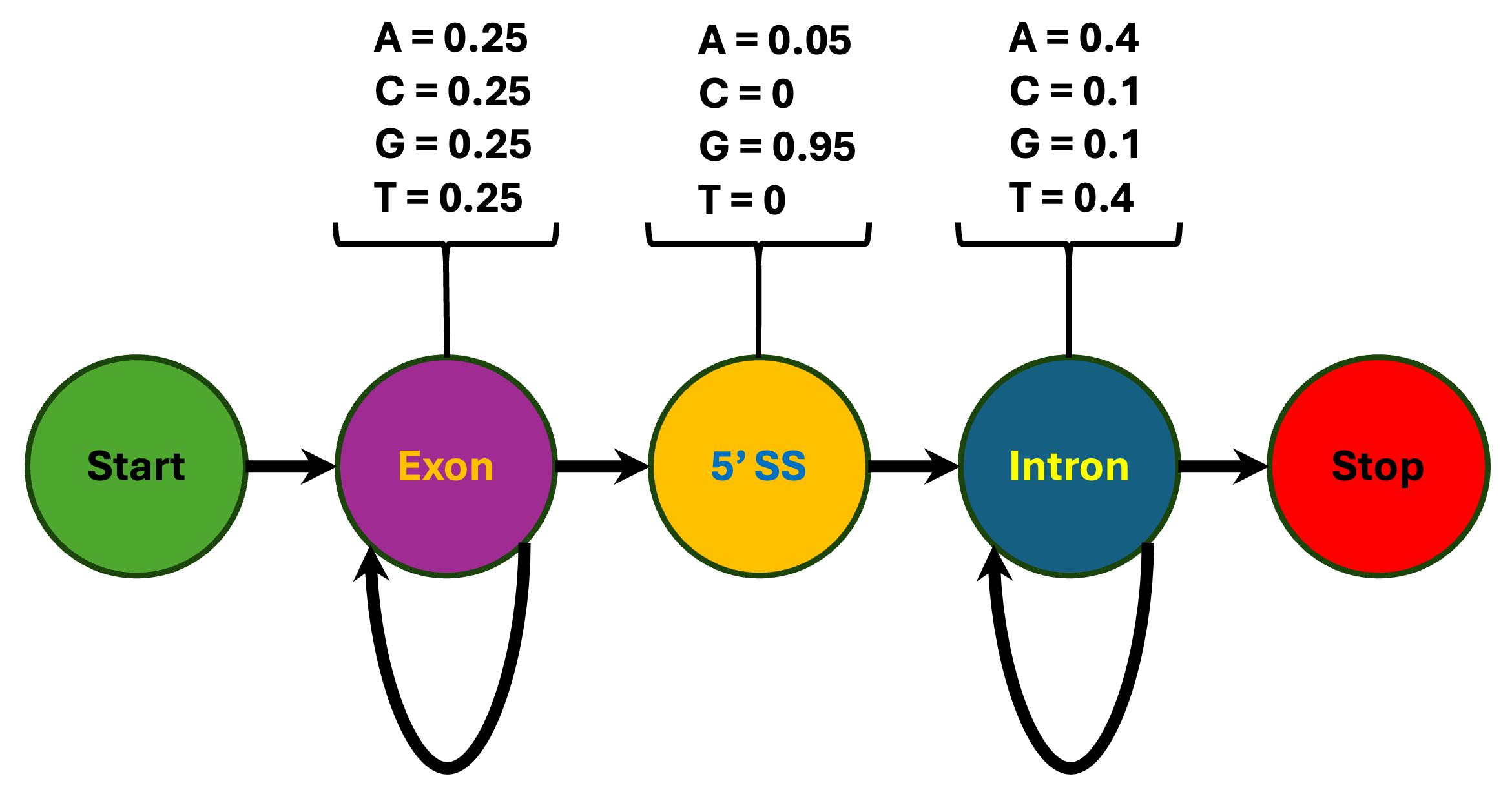
To see how HMMs work in practice, consider a simplified example of identifying splice sites in eukaryotic genes. Suppose we have a DNA sequence that begins in an exon, contains one 5′ splice site, and ends in an intron. The biological question is straightforward: where does the transition from exon to intron occur? Different regions of genes have distinct statistical properties that we can exploit. Exons might display roughly uniform base composition, introns tend to be AT-rich, and the consensus nucleotide at the 5′ splice site is almost always a G1. An HMM for this problem would contain three states corresponding to these three functional categories: exon, splice site, and intron. Each state would be characterized by emission probabilities that reflect the expected base composition for that functional class, and transition probabilities that describe the linear order in which we expect to encounter these states as we move along the sequence1,5. Because this is an ordered sequence we can add a start and stop state to either end as shown in Figure 9.1.
A toy hidden Markov model (HMM) for a simple eukaryotic gene with one exon and one intron. The model has four emitting states—Exon, 5′ splice site (5′ SS), Intron, and Stop—plus non-emitting Start and Stop states. Each emitting state is associated with a nucleotide emission distribution (shown above the state), and arrows between states indicate transition probabilities. The Exon and Intron states have high self-transition probabilities (0.9), reflecting variable-length coding and intronic regions, whereas transitions from Exon to 5′ SS and from Intron to Stop occur with lower probability (0.1), modeling rare boundary events. This compact model illustrates how HMMs can encode both sequence composition and gene structure in a single probabilistic framework, following the teaching example in Weisstein et al. (2021)5.
When an HMM generates a sequence, it produces two parallel streams of information. One is the state path—the sequence of hidden states visited during generation—which corresponds to the biological labels we ultimately want to assign. The other is the observed sequence itself, with each nucleotide emitted according to the emission probabilities of whatever state the model occupied at that position. The state path forms a Markov chain because the choice of the next state depends only on the current state, not the entire history. Since we typically observe only the nucleotide sequence and not the underlying state path, this state sequence is hidden, giving the model its name1.
Several fundamental concepts appear repeatedly when working with HMMs. The states of an HMM represent the hidden functional categories or labels we wish to assign to sequence positions. Each state is characterized by two types of probabilities. Emission probabilities \(e(x|i)\) specify the probability that state \(i\) will produce symbol \(x\), and these probabilities must sum to one across all possible symbols. Transition probabilities \(t(i,j)\) describe the probability of moving from state \(i\) to state \(j\), and these also must sum to one across all possible destination states1,2. A basic explanation using the example of weather is provided as a video introduction to these concepts.
The collection of all states, emission probabilities, and transition probabilities fully specifies an HMM. The joint probability that an HMM with parameters \(\theta\) generates both a particular state path \(\pi\) and an observed sequence \(S\) is the product of all the relevant emission and transition probabilities. Because HMMs are fully probabilistic models, we can use standard tools from probability and statistics to manipulate these quantities, optimize parameters, and interpret scores as probabilities rather than arbitrary units1.
In practice, we can now use the toy gene model in Figure 9.1 to score concrete hypotheses about how an observed sequence was generated. For example, given the sequence CTTCATGTGAAAGCAGACGTAAGTCA, one candidate explanation is that all bases before the splice site come from the Exon state, the splice dinucleotide comes from the 5′ SS state, and all remaining bases come from the Intron state, corresponding to the state path EEEE…E5II…I shown in Figure 1 of Eddy 20041. The probability of this particular path is obtained by multiplying the appropriate transition probabilities (for example, the repeated Exon→Exon self-transitions, followed by Exon→5′ SS and 5′ SS→Intron) and emission probabilities for each base in the sequence given its state, and then taking the log to obtain the log P reported in the right margin. We conceptually repeat this calculation for every possible state path that could generate the sequence and select the most likely one (the path with the highest probability, or equivalently the least negative log P), which in this toy example identifies the most probable 5′ splice site position1.
Constructing an HMM begins by specifying the symbol alphabet (for example, A, C, G, and T for DNA), the number and types of states in the model, the emission probabilities associated with each state, and the transition probabilities between states2. Any model satisfying these basic properties qualifies as an HMM, which means that designing a new model often reduces to drawing an intuitive picture that represents the biological system of interest1. This graphical simplicity makes HMMs a natural fit for building complex models of gene structure, protein families, or evolutionary processes4.
Hidden Markov Models for Gene Prediction
One of the most successful applications of HMMs in computational biology is the prediction of gene structures in genomic sequences4. The challenge of computational gene finding is far from trivial, particularly in eukaryotes where genes are typically interrupted by introns that can span thousands of base pairs. Early gene prediction programs relied on simple pattern matching or sliding window approaches, but these methods struggled to integrate multiple sources of information and often produced inconsistent predictions with high false positive rates4.
The introduction of HMM-based gene finders transformed the field by providing a principled statistical framework for combining diverse signals—splice site consensus sequences, codon usage bias, exon and intron length distributions, and open reading frame constraints—into a single coherent model2,4. Rather than building an ad hoc scoring system, we specify how likely it is that coding regions emit given DNA patterns, how often splice sites occur, and how exons and introns are arranged. The HMM then computes the most probable gene structure consistent with the observed sequence and model parameters.
Generalized HMMs and Gene Structure
Most modern gene prediction programs employ a variant of HMMs called generalized hidden Markov models (GHMMs). While ordinary HMMs emit a single symbol per state, GHMMs allow each state to emit a sequence of variable length. This modification is essential for gene finding because functional elements like exons and introns span multiple nucleotides, and their lengths vary considerably from one instance to another4.
In a GHMM for gene prediction, states correspond to biological features such as exons, introns, splice donor regions, splice acceptor regions, and intergenic sequences. Each state is associated with a probability model that describes both the composition and the length distribution of sequences that the state can emit4. For example, exons are modeled using codon statistics that reflect nonuniform codon usage, while introns may be modeled with simpler background nucleotide distributions and length distributions that match the organism’s intronic architecture2.
Splice sites provide a concrete illustration of this modeling strategy. The first few nucleotides at intron boundaries show strong position-specific preferences. In many eukaryotes, the canonical donor site begins with the dinucleotide GT, and the third and fourth positions show characteristic biases toward purines and adenine, respectively4. By compiling these position-specific frequencies from a training set of confirmed splice sites, we can build a weight matrix model that assigns a probability to any candidate splice site sequence. In the GHMM, this weight matrix becomes the emission model for the splice donor state and helps distinguish true splice sites from spurious GT dinucleotides elsewhere in the genome4.
The middle regions of exons and introns require other probability models. For exon states, gene finders typically model the sequence using a probabilistic description that captures codon usage bias and period-3 base composition patterns2. One common approach uses separate states for the first, second, and third positions of codons, each with its own emission probabilities. For intron states, the model might use a simpler background nucleotide distribution, with emission probabilities estimated from intronic training sequences. Length distributions for exons, introns, and intergenic regions are also modeled, often using geometric or more flexible distributions tailored to the organism4.
Dual-genome and multi-genome de novo gene predictors extend this idea by using alignments between a target genome and one or more related “informant” genomes4. Instead of treating the observed data as a single DNA sequence, these methods model aligned pairs (or tuples) of nucleotides and indels, allowing them to leverage evolutionary conservation to improve gene predictions. Conserved coding regions show characteristic patterns in alignments, such as mismatches that preserve amino acid sequences or gaps that maintain reading frame, and these patterns can be encoded in the emission models of a GHMM2,4.
AUGUSTUS and Constraint-Based Annotation
AUGUSTUS is a widely used gene prediction system that exemplifies the power and flexibility of GHMM-based gene finding3. At its core, AUGUSTUS models the sequence around splice sites, branch point regions, translation start sites, coding regions, non-coding regions, and the length distributions of exons, introns, and intergenic regions. The model is trained on known genes from a given species, producing species-specific parameter sets that capture typical gene architecture3.
Beyond its probabilistic modeling, AUGUSTUS introduces an important practical feature: the ability to incorporate user-defined constraints. Users can specify positions of known exons, introns, splice sites, translation start sites, or stop codons, based on experimental evidence or other computational predictions3. The system then searches for the most probable gene structure that is consistent with these constraints. This capability is particularly valuable when partial experimental data (such as an RT-PCR-validated intron or an expressed sequence tag alignment) is available. Rather than ignoring such data or relying on manual interpretation alone, AUGUSTUS integrates it directly into the probabilistic framework. This combination of a rich probabilistic model and constraint-based refinement makes AUGUSTUS an ideal tool for bridging the gap between fully automated and manual annotation3,4.
In Lab 6, you will be working with a toy model of ab initio gene prediction. Similarly, in your Manual Annotation Project, you will be working with the homology-based annotation tool using GeneWise. AUGUSTUS can be viewed as a natural extension of those ideas to full-genome scale, providing a realistic context for understanding how HMMs underpin modern annotation pipelines3.
Manual vs. Automated Annotation
The distinction between manual and automated gene annotation reflects a fundamental tension in genomics between throughput and accuracy4. Automated annotation pipelines use computational gene finders like AUGUSTUS to generate predictions across entire genomes, enabling the rapid processing of newly sequenced species. These automated predictions serve as crucial starting points for functional genomics studies and can be updated as new evidence becomes available3.
Manual annotation, by contrast, involves human curators examining computational predictions in the context of multiple lines of evidence, including expressed sequence tag alignments, protein homology, RNA-seq data, and comparative genomics information4. Curators use this evidence to refine gene models, identify alternative splice forms, and resolve ambiguous cases where computational methods disagree. This process is time-consuming and expensive, but it generally produces more accurate gene structures than purely computational approaches4.
The most reliable annotation strategy combines both approaches. Automated gene finders provide initial predictions, which are then manually curated for genes of particular interest or in cases where multiple predictions conflict. In your laboratory work, when you manually annotate genes using GeneWise, you are effectively acting as a human integrator of evidence, complementing the purely statistical reasoning embodied by HMM-based gene finders.
Profile Hidden Markov Models
While the basic HMM architecture works well for many sequence analysis problems, biological sequences often display position-specific patterns that require more specialized models. Profile hidden Markov models, or profile HMMs, address this need by representing the consensus properties of a multiple sequence alignment2. Rather than modeling individual sequences, profile HMMs capture the statistical patterns that characterize an entire family of related sequences, making them particularly powerful for tasks like protein family classification, remote homology detection, and motif discovery.
The architecture of a profile HMM differs from general-purpose HMMs in its strictly linear, left-to-right structure without cycles. The model repetitively uses three types of states to describe each position in the alignment. Match states represent conserved positions in the alignment, with emission probabilities reflecting the observed base or amino acid frequencies at that position. Insert states handle additional residues that appear in some sequences but not others, accommodating length variation among family members. Delete states are silent, non-emitting placeholder states that allow sequences to skip conserved positions, thereby modeling deletions relative to the consensus2.
Constructing a profile HMM from a multiple sequence alignment is conceptually straightforward. Consider an alignment with a certain number of columns representing a conserved domain or motif. For each column, we must decide whether it should be modeled by a match state or an insert state. A simple heuristic compares the number of residues to the number of gaps in each column: if residues outnumber gaps, we treat the column as a conserved position represented by a match state, and any gaps are modeled by the corresponding delete state. If gaps outnumber residues, we view the residues as insertions and represent the column with an insert state. Once we have assigned state types to all columns, we estimate emission probabilities by counting the frequency of each symbol at each position, and we estimate transition probabilities by counting state-to-state transitions across the sequences in the alignment, often with pseudocounts to avoid zero probabilities2.
Profile HMMs have become workhorses of modern protein sequence analysis2. Software packages such as HMMER and SAM provide complete toolkits for building profile HMMs from alignments, searching sequence databases with profile HMMs, and comparing new sequences against libraries of pre-built models. Large-scale resources like the Pfam database and PROSITE have compiled profile HMMs for thousands of known protein domains and families, enabling rapid functional annotation of newly sequenced proteins. When a researcher obtains a new protein sequence of unknown function, searching it against Pfam can reveal which known domains it contains, providing immediate insights into its likely biochemical activities and cellular roles2.
The applications of profile HMMs extend beyond simple sequence searches. Comparing two profile HMMs—representing two different multiple alignments or sequence families—can detect remote homology relationships that would be missed by pairwise sequence comparison2. Tools such as HHsearch generalize traditional pairwise alignment algorithms to find optimal alignments between pairs of profile HMMs, greatly extending the depth of homology detection. Researchers have also adapted profile HMMs to model non-sequence features, such as protein secondary structure patterns, where the model emits secondary structure symbols (helix, strand, coil) rather than amino acids. These secondary-structure profile HMMs can recognize three-dimensional protein folds based solely on predicted secondary structure, demonstrating the versatility of the HMM framework2.
Pair Hidden Markov Models
While profile HMMs model a family of related sequences, pair hidden Markov models, or pair HMMs, address the fundamental problem of comparing two individual sequences2. Sequence alignment is central to nearly all biological sequence analysis, as the degree of similarity between sequences often indicates functional or evolutionary relationships. Pair HMMs provide a formal probabilistic framework for finding sequence alignments, computing alignment probabilities, and evaluating the significance of aligned regions2.
The key innovation of pair HMMs is that they simultaneously generate two aligned sequences rather than a single sequence. Consider a simple pair HMM with three states. An insert state for sequence 1 emits a single symbol in the first sequence but nothing in the second sequence, representing an insertion in the first sequence or, equivalently, a deletion in the second. Similarly, an insert state for sequence 2 emits a symbol only in the second sequence. A match/mismatch state emits a pair of symbols, one in each sequence, representing positions that are aligned to each other. As the model transitions among these three states, it builds up a pairwise alignment between the two output sequences2.
There is a one-to-one correspondence between a pair HMM state path and a sequence alignment. Each state in the path specifies whether the current position in each sequence is emitted as an aligned pair or as an insertion in one sequence or the other. This means that finding the optimal alignment between two sequences is mathematically equivalent to finding the optimal state path through a pair HMM. A modification of the Viterbi dynamic programming algorithm can find this optimal path efficiently, with computational complexity proportional to the product of the two sequence lengths2. This approach recovers alignments comparable to those produced by classical dynamic programming algorithms, but the pair HMM framework provides additional capabilities that standard alignment methods lack.
One major advantage of pair HMMs is their ability to compute the overall probability that two sequences are related, rather than simply identifying a single best alignment. When sequences are weakly similar, there may be many plausible alignments with similar scores, and focusing on only the optimal alignment can be misleading. The pair HMM framework allows us to sum the probabilities over all possible alignments to obtain the total probability of observing the two sequences given the model. This calculation can be performed efficiently using a modified version of the forward algorithm. Additionally, pair HMMs can compute position-specific alignment probabilities, quantifying the probability that any particular pair of residues are aligned to each other across all possible alignments. These posterior probabilities provide a natural measure of alignment confidence and can identify regions where the alignment is uncertain2.
Pair HMMs have found extensive applications beyond basic pairwise alignment. Many state-of-the-art multiple sequence alignment programs, including ProbCons, use pair HMMs as a core component2. ProbCons employs a pair HMM to compute posterior probabilities for all pairwise alignments among the input sequences, then uses these probabilities to guide the progressive assembly of the full multiple alignment. Instead of directly using the optimal Viterbi alignment for each sequence pair, ProbCons identifies the alignment that maximizes the expected number of correctly aligned positions based on the posterior probabilities. The algorithm further improves accuracy by incorporating a probabilistic consistency transformation, which considers information from alignments to intermediate sequences when scoring each pairwise alignment. This consistency-based approach has demonstrated substantial improvements over traditional progressive alignment methods and has influenced the design of subsequent multiple alignment tools2.
In Chapter 5, we explored various algorithms for multiple sequence alignment, a fundamental challenge in comparative genomics and evolutionary analysis. ProbCons represents a significant advance in this area by leveraging pair HMMs to bring probabilistic rigor to the alignment process2. Traditional progressive alignment methods construct multiple alignments by iteratively combining pairwise alignments according to a guide tree, but they lack a principled framework for quantifying alignment uncertainty or propagating information across multiple sequences.
ProbCons addresses these limitations through three key innovations. First, it uses a pair HMM to compute posterior alignment probabilities for all sequence pairs, providing a confidence estimate for each potential aligned position. Second, it applies probabilistic consistency transformation, which refines pairwise alignment scores by considering paths through intermediate sequences. If sequence A aligns well to sequence C, and sequence C aligns well to sequence B, this provides additional evidence that A and B should be aligned in a consistent manner. Third, ProbCons uses these refined scores to identify alignments that maximize expected accuracy rather than simply optimizing a scoring function.
The performance improvements from ProbCons have been substantial, particularly for divergent sequences where alignment uncertainty is high. This probabilistic framework has become a template for modern multiple alignment algorithms and exemplifies how HMM-based approaches can elevate the quality and reliability of fundamental bioinformatics operations2.
Pair HMMs also play a central role in comparative gene prediction. Algorithms such as SLAM and TWAIN use generalized pair HMMs to simultaneously compare two genomic sequences and annotate their gene structures. These methods combine the alignment capabilities of pair HMMs with the gene structure modeling of gene-finding HMMs, creating integrated models that can leverage conservation patterns between species to improve gene prediction accuracy2. The resulting predictions are typically more accurate than single-genome gene finders because evolutionary conservation provides strong evidence for functional elements.
Other Extensions and Applications
Beyond gene prediction and sequence alignment, HMMs have proven valuable for analyzing biological sequences with more complex structural and evolutionary features2. RNA sequences present particular challenges because their function depends not only on primary sequence but also on secondary structure, which arises from base pairing interactions between distant positions. Standard HMMs assume that each emission depends only on the current state, making it difficult to model the long-range correlations induced by base pairing. Several extensions to the basic HMM framework have been developed to address this limitation2.
Context-sensitive HMMs (csHMMs) extend the HMM architecture by allowing certain states to use contextual information from previous emissions when determining emission probabilities. The model includes three types of states: standard single-emission states, pairwise-emission states that store emitted symbols in memory, and context-sensitive states that retrieve stored symbols and adjust their emission probabilities accordingly. For modeling RNA secondary structures, pairwise-emission states can be placed at positions where one half of a base pair occurs, storing the emitted base for later use. When the model reaches the complementary base-pairing position, a corresponding context-sensitive state retrieves the stored base and emits a complementary nucleotide with high probability. This mechanism allows csHMMs to represent a wide range of base-pairing patterns, including certain complex structures such as pseudoknots2.
Profile context-sensitive HMMs (profile-csHMMs) combine the RNA modeling capabilities of csHMMs with the profile representation of multiple alignments. These models can represent the conserved sequence features and base-pairing patterns that characterize families of functional RNAs. Constructing a profile-csHMM from an RNA alignment with structural annotation is analogous to building a standard profile HMM, but match states can be designated as single-emission, pairwise-emission, or context-sensitive depending on whether they represent unpaired positions or the two sides of conserved base pairs. Profile-csHMMs have been applied to RNA homology searches and structural alignment, providing powerful tools for analyzing non-coding RNAs2.
The computational cost of RNA analysis with sophisticated HMM variants can be substantial, as modeling base-pairing interactions typically requires algorithms with cubic time complexity or worse. Various acceleration strategies have been developed to make these methods practical for genome-scale searches. One effective approach uses standard profile HMMs, which consider only sequence information and run quickly, to prescreen a database and filter out sequences that are unlikely to match the full structural model. The more expensive structure-aware model is then applied only to sequences that pass the initial filter, dramatically reducing the average computational cost while maintaining high sensitivity2.
HMMs for Local Ancestry and Association Studies
Another important application domain for HMMs is local ancestry inference in admixed populations. When individuals have genetic ancestry from multiple continental populations, their genomes become mosaics of chromosomal segments inherited from different ancestral groups. HMM-based methods can model this mosaic as a sequence of hidden ancestry states along the genome, with the observed genotypes (or haplotypes) providing evidence about which ancestry is most likely at each position2,6.
In a typical local ancestry HMM, the hidden states correspond to ancestry labels (for example, African, European, Indigenous American), and the emission probabilities describe the likelihood of observing the genotypes in a given segment assuming each possible ancestry, given reference panels from those populations6. Transition probabilities between ancestry states reflect recombination, with higher recombination rates leading to more frequent ancestry switches. Once local ancestry has been inferred, these segment-level assignments can be integrated into genetic association analyses, admixture mapping, and polygenic risk score construction to improve power and interpretability in diverse populations6.
Recent reviews highlight both the opportunities and challenges of local ancestry-based association studies, including issues of reference panel selection, model misspecification, and computational scaling as sample sizes grow6. Nevertheless, the HMM framework remains central because it provides a flexible way to combine recombination models, ancestry information, and genotype likelihoods within a coherent probabilistic system.
Hidden Markov models have recently illuminated one of the most fascinating questions in human evolutionary history: the extent and timing of interbreeding between modern humans and Neanderthals. As modern humans migrated out of Africa and encountered Neanderthal populations in Eurasia, genetic material was exchanged through interbreeding, leaving traces of Neanderthal ancestry in the genomes of present-day non-African populations7,8. Identifying these introgressed segments and studying their properties over time requires sophisticated computational methods to distinguish Neanderthal ancestry from the predominant modern human background.
Two recent studies approached this problem using HMM-based local ancestry methods on ancient and present-day genomes. Iasi et al. used a specialized HMM called admixfrog to catalog Neanderthal ancestry segments in more than 300 ancient and present-day human genomes spanning the past 50,000 years7. The method employs an HMM where each genomic window can be assigned to one of three ancestries: Neanderthal, Denisovan (another archaic human group), or modern human. The model uses high-coverage Neanderthal and Denisovan genomes and a panel of present-day African individuals as references representing these ancestry sources. For each target individual, the HMM evaluates small genomic windows and estimates the most likely ancestry based on the pattern of alleles present and their frequencies in the reference populations7.
In parallel, Sümer et al. analyzed some of the earliest modern human genomes outside Africa to constrain the timing of Neanderthal admixture events8. By combining HMM-based identification of archaic segments with demographic modeling, they showed that early modern humans carried long, distinctive Neanderthal segments that are not fully shared with present-day non-Africans, pointing to multiple introgression events and helping to narrow the window during which Neanderthal gene flow occurred8. Together, these studies illustrate how applying HMMs to both ancient and present-day genomes allows researchers to disentangle complex admixture histories and relate them to archaeological evidence.
The work by Iasi et al. revealed that the vast majority of Neanderthal ancestry in modern humans derives from a single extended period of gene flow that occurred between roughly 50,500 and 43,500 years ago in the common ancestors of all non-African populations7. This conclusion emerged from several lines of evidence enabled by the HMM analysis. First, Neanderthal segments are extensively shared among present-day populations, with the sharing patterns reflecting the overall population structure of modern humans rather than indicating independent admixture events. Second, the Neanderthal segments in post-Ice Age individuals show similar levels of divergence from sequenced Neanderthal genomes, consistent with introgression from a single or closely related group. Third, by measuring how Neanderthal segments decay in length over time due to recombination, the researchers could estimate both the timing and duration of the admixture period7.
The HMM framework also enabled the researchers to study natural selection on Neanderthal ancestry by tracking how the frequency of introgressed segments changed over time. They identified genomic regions where Neanderthal variants rose to high frequency rapidly, suggesting positive selection for beneficial alleles affecting skin pigmentation, metabolism, and immune function7. Conversely, they found that genomic regions depleted of Neanderthal ancestry—so-called “archaic deserts”—were established almost immediately after the gene flow event, indicating strong negative selection against Neanderthal variants in functionally constrained regions. The X chromosome showed an especially striking pattern, with large deserts of Neanderthal ancestry overlapping regions that experienced selective sweeps in non-African populations7,8.
This case study illustrates how HMMs can address complex questions in population genetics by formally modeling the mosaic ancestry structure of admixed genomes. The ability to assign ancestry to small genomic segments, quantify uncertainty in these assignments, and track changes in ancestry patterns over time has transformed our understanding of human evolutionary history and adaptation6–8.
The Connection Between HMMs and MCMC
Hidden Markov models and Markov chain Monte Carlo (MCMC) methods share conceptual foundations in Markov chains, but they serve fundamentally different roles in computational biology2. HMMs are generative models that describe how observed sequences are produced by underlying state sequences, and we use them to infer the most likely hidden states or to compute probabilities of observed data1. MCMC, by contrast, is a computational technique for drawing samples from complex probability distributions that cannot be analyzed analytically, and it plays a central role in Bayesian inference and statistical modeling2.
The connection becomes clearest when considering parameter estimation for HMMs. When we have a collection of related sequences and want to build an HMM that represents them, we need to estimate the transition probabilities, emission probabilities, and sometimes the structure of the model itself. The Baum–Welch algorithm, which is an expectation–maximization (EM) approach, provides one standard method for parameter estimation1,2. However, EM algorithms can be sensitive to local optima and may not fully characterize uncertainty in parameter estimates.
Bayesian approaches to HMM parameter estimation use MCMC methods to sample from the posterior distribution of model parameters given the observed sequences. Rather than finding a single best set of parameters, MCMC methods generate many parameter sets drawn from their posterior probability distribution, naturally quantifying uncertainty and avoiding over-commitment to local optima. The Markov chain in MCMC refers to a sequence of parameter configurations where each new configuration is proposed based only on the current configuration, satisfying the Markov property. By carefully designing the proposal mechanism and acceptance criteria, MCMC algorithms ensure that the chain eventually explores parameter space in proportion to the posterior probability, providing valid statistical inference2.
Monte Carlo EM algorithms represent a hybrid approach that uses sampling to approximate difficult-to-compute expectations within the EM framework. When working with complex HMMs where computing exact expectations is intractable, MCEM uses Monte Carlo sampling to approximate these quantities, enabling parameter estimation for broader classes of models2. This interplay between HMMs and MCMC methods highlights how different computational techniques can be combined to address challenging problems in biological sequence analysis.
Practice Problem Sets
Basic HMM Concepts: Consider a simple HMM with two states: C (CpG island) and N (non-CpG island). The emission probabilities for state C give equal probability (0.25) to all four nucleotides, while state N is AT-rich with \(e_N(A) = e_N(T) = 0.35\) and \(e_N(C) = e_N(G) = 0.15\). The transition probability from C to N is 0.1, and from N to C is 0.05. Calculate the probability that this HMM generates the sequence ACGT starting in state C and ending in state N along the state path C–C–C–N.
Gene Finding with GHMMs: Explain why generalized hidden Markov models are more appropriate than standard HMMs for eukaryotic gene prediction. What specific biological features of genes necessitate the variable-length emissions allowed by GHMMs? How would you modify a GHMM to model alternative splicing?
Profile HMM Construction: Given a multiple sequence alignment with seven columns, three sequences, and the following pattern:
Seq1: ACGT-GA
Seq2: ACG--GA
Seq3: ACGTTGA
Determine which columns should be represented by match states versus insert states using a simple gap/residue heuristic. Sketch the resulting profile HMM structure and estimate the emission probabilities for the match states.
Pair HMM Alignment: A pair HMM for protein sequence alignment has three states: M (match/mismatch), X (insert in sequence 1), and Y (insert in sequence 2). If you observe an alignment of length 10 that contains 7 matched positions and 3 positions where residues in sequence 1 are gapped, write out a plausible state path through the pair HMM. How does this state path correspond to the standard representation of a gapped alignment?
Model Selection: You have built two different HMMs to model a protein family—one simple model with 15 states and one complex model with 45 states. The complex model achieves higher likelihood on your training sequences. What concerns might you have about using the complex model for searching databases? How could you evaluate which model generalizes better to new sequences?
RNA Secondary Structure: Context-sensitive HMMs can model base-pairing interactions by using memory to store emitted bases and later retrieve them at complementary positions. Sketch a csHMM that could model a simple hairpin structure with a 6-nucleotide stem (three base pairs) and a 4-nucleotide loop. Label the states as pairwise-emission, context-sensitive, or single-emission, and indicate which states use memory.
Reflection Questions
Integration of Evidence: In your Manual Annotation Project, you performed manual gene annotation using GeneWise to make homology-based predictions. Reflect on how an HMM-based gene finder like AUGUSTUS integrates different types of evidence (splice signals, codon bias, length distributions). What are the advantages and limitations of having the computer automatically weight these different information sources compared to a human curator making judgment calls? When might you trust the HMM more than your own assessment, and when might your expert judgment carry more weight?
The Hidden Information Problem: Throughout this chapter, we emphasized that HMMs model two parallel processes—a visible sequence and a hidden state path. Think about other biological problems beyond those discussed where you observe some data but care primarily about hidden underlying processes. For example, consider ChIP-seq data showing protein–DNA binding across a genome, or Hi-C data showing chromosome conformation. Could HMMs be useful for these problems? What would the states represent? What would the observations be?
Probabilistic vs. Deterministic Approaches: Compare the HMM framework to simpler, deterministic approaches for sequence analysis, such as scanning for exact motif matches or using fixed score thresholds. What are the conceptual and practical advantages of a fully probabilistic approach? In what situations might a simpler deterministic method actually be preferable despite being less statistically sophisticated?
Model Design and Biological Understanding: One appealing feature of HMMs is that designing a model often involves drawing an intuitive picture. Reflect on whether this simplicity could be a double-edged sword. Does the ease of sketching an HMM architecture risk oversimplifying biology? How would you guard against building models that are mathematically elegant but biologically unrealistic?
Ancient DNA and Temporal Genomics: The Neanderthal ancestry case study illustrates how ancient DNA provides a time series of genomic data. How does having observations from multiple time points fundamentally change what we can infer about evolutionary processes? Consider other questions in evolutionary biology or medical genetics where access to historical samples might provide decisive evidence. What are the practical and ethical challenges of obtaining such samples?
The Limits of HMMs: We mentioned that HMMs struggle with long-range correlations because each emission depends only on the current state. Yet we have seen various workarounds—context-sensitive states for RNA, triplet-emitting states for codons. Reflect on whether these extensions maintain the conceptual elegance of HMMs or whether they indicate that fundamentally different approaches (like deep learning models) might be needed for some problems. What would we lose by abandoning the HMM framework, and what might we gain?