Let’s try the plot again:
pva$Programming.Language. <- as.factor(pva$Programming.Language.)
plot(pva$Programming.Language.,pva$Sys.Run.Time.)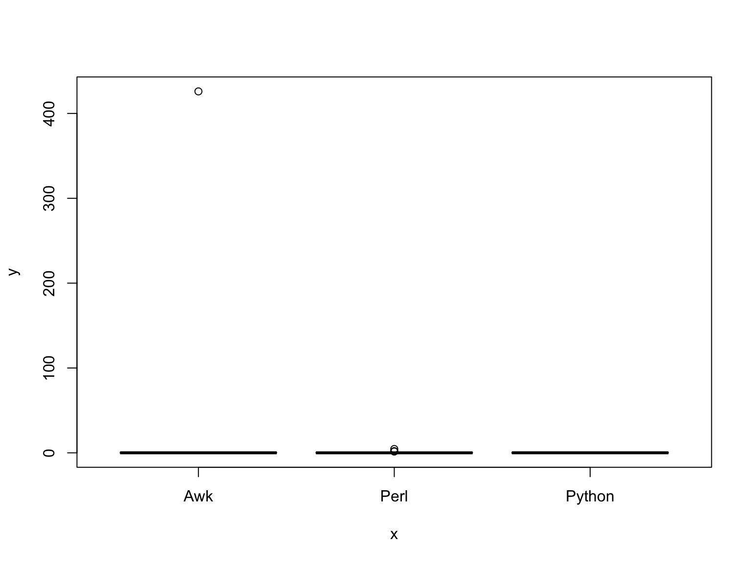
Now, we have a box plot of each dataset.
What modification could you make to better visualize this plot?
Laurie Stevison & Amanda Clark
If you are using this code with the video, note that some slides have been added post-recording and are not shown. See walkthrough2.R in the compressed data tarball for the code from the recording.
For this tutorial we will be working with the “Lab6_Perl_v_Awk.csv” “BodyFat.csv” datasets.
Make an R Notebook for this walk-through tutorial to save all the code you will be learning. We will cover:
aovglmYou are working within an R project (check in the top right corner of RStudio - you should see the project name “R_Mini_Course”).
This means that the project directory will also be set as working directory. The exception is in a R Notebook, where the working directory is where the R Notebook is saved.
You should be saving your notebooks in the R Project and using
../.. to point at the main project directory.
Before starting, it may be helpful to have a chunk of code that does the following:
rm(list=ls())library(<package-name>)sessionInfo()list.files(getwd())Our first dataset will be a summary of results from Lab #6: A comparisons of awk and perl.
You will need to add path information to the raw_data
directory once you have uncompressed the data tarball.
Read “Lab6_Perl_v_Awk.csv” into an object called
pva:
Read “BodyFat.csv” into an object called fat:
You may also read in the previously made object:
##   ID     Start.time Completion.time Operating.System...i.e..iOS..Ubuntu. Programming.Language.
## 1  2 10/19/20 16:05  10/19/20 16:29                                  IOS                   Awk
## 2  3 10/19/20 17:56  10/19/20 17:58                               Mac OS                  Perl
## 3  4 10/19/20 17:58  10/19/20 17:58                               Mac OS                   Awk
##   Sys.Run.Time. Input.VCF.File.Size.
## 1            na                 Full
## 2         0.031                 Full
## 3 0.03 Full## IDNO BODYFAT DENSITY AGE WEIGHT HEIGHT ADIPOSITY NECK CHEST ABDOMEN HIP THIGH KNEE ANKLE
## 1 1 12.6 1.0708 23 154.25 67.75 23.7 36.2 93.1 85.2 94.5 59.0 37.3 21.9
## 2 2 6.9 1.0853 22 173.25 72.25 23.4 38.5 93.6 83.0 98.7 58.7 37.3 23.4
## 3 3 24.6 1.0414 22 154.00 66.25 24.7 34.0 95.8 87.9 99.2 59.6 38.9 24.0
## BICEPS FOREARM WRIST X
## 1 32.0 27.4 17.1 NA
## 2 30.5 28.9 18.2 NA
## 3 28.8 25.2 16.6 NAClick the data object in the environment tab in RStudio…
Notice these five columns of data:
ID (Student)Sys.Run.Time. (Run Time)Programming.Language. (e.g. Perl; Awk)Input.VCF.File.Size (Partial/Full File)Operating.System...i.e..iOS..Ubuntu. (OS)We also have some missing data.
Let’s compare the distribution of run times for each language.
Notice, the plot looks unexpected or it did not plot at all. That is because we have some missing data and columns that have not been coded correctly.
If you are reading in the raw data, we can read the data in again - specifying that the string “na” should be coded as missing data and columns with strings should be treated as factors (this means that these columns can be summarized into categories or levels).
dplyr PracticeIf you are reading in the saved data object in the beginning, let’s
get some extra practice with dplyr (introduced in Module 3)
to perform these same modifications, step-by-step.
##   ID     Start.time Completion.time Operating.System...i.e..iOS..Ubuntu. Programming.Language.
## 1  2 10/19/20 16:05  10/19/20 16:29                                  IOS                   Awk
## 2  3 10/19/20 17:56  10/19/20 17:58                               Mac OS                  Perl
## 3  4 10/19/20 17:58  10/19/20 17:58                               Mac OS                   Awk
##   Sys.Run.Time. Input.VCF.File.Size.
## 1          <NA>                 Full
## 2         0.031                 Full
## 3          0.03                 Full
Notice the “na” strings are now properly coded as NAs (compare with
slide 5). If you run summary on the object, we still have the issue of
Sys.Run.Time. being coded as “character” data.
Let’s see how we can fix that on the next slide…
##        ID      Start.time        Completion.time    Operating.System...i.e..iOS..Ubuntu.
##  Min.   : 2   Length:37          Length:37          Length:37
##  1st Qu.:11   Class :character   Class :character   Class :character
##  Median :20   Mode  :character   Mode  :character   Mode  :character
##  Mean   :20
##  3rd Qu.:29
##  Max.   :38
##
##  Programming.Language. Sys.Run.Time.      Input.VCF.File.Size.
##  Length:37             Min.   :  0.0000   Length:37
##  Class :character      1st Qu.:  0.0160   Class :character
##  Mode  :character      Median :  0.0490   Mode  :character
##                        Mean   : 14.0506
##                        3rd Qu.:  0.1205
##                        Max.   :426.0000
##                        NA's   :6
Fixed! Lastly, we want to make sure the other columns are treated as categorical.
Here, we are specifying two columns to be treated as categorical
(i.e., mutate the data across Programming.Language. &
Input.VCF.File.Size. by coding them factors).
Remember the %>% symbol from magrittr (tidyverse) is
a pipe.
Use summary to see the changes made to the two columns
of data we converted to factors.
We could convert all “character” columns to factors by replacing
...across(c(<columns>, <targeted>),...
with
...across(where(is.character),...
Let’s try the plot again:
pva$Programming.Language. <- as.factor(pva$Programming.Language.)
plot(pva$Programming.Language.,pva$Sys.Run.Time.)
Now, we have a box plot of each dataset.
What modification could you make to better visualize this plot?
Let’s revisit some basic summary statistics for this dataset.
##        ID      Start.time        Completion.time    Operating.System...i.e..iOS..Ubuntu.
##  Min.   : 2   Length:37          Length:37          Length:37
##  1st Qu.:11   Class :character   Class :character   Class :character
##  Median :20   Mode  :character   Mode  :character   Mode  :character
##  Mean   :20
##  3rd Qu.:29
##  Max.   :38
##
##  Programming.Language. Sys.Run.Time.      Input.VCF.File.Size.
##  Awk   :13             Min.   :  0.0000   Full   :22
##  Perl  :18             1st Qu.:  0.0160   Partial:15
##  Python: 6             Median :  0.0490
##                        Mean   : 14.0506
##                        3rd Qu.:  0.1205
##                        Max.   :426.0000
##                        NA's   :6
Notice the range for mean run time is quite skewed. Let’s look at the overall distribution
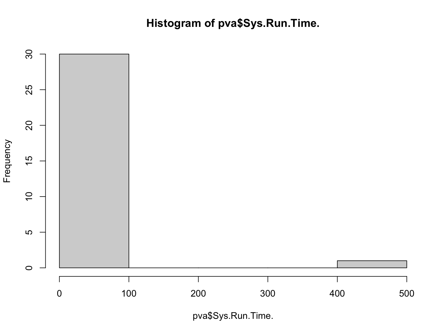
Because the majority of our observations are less than 1 and some folks may have put actual run time instead of SysRunTime, let’s go ahead and exclude these extreme values and look at the boxplot again:
pva2=subset(pva,pva$Sys.Run.Time.<=1)
plot(pva2$Programming.Language.,pva2$Sys.Run.Time.,main="Perl versus Awk",xlab="Programming Language",ylab="Sys Time in Seconds")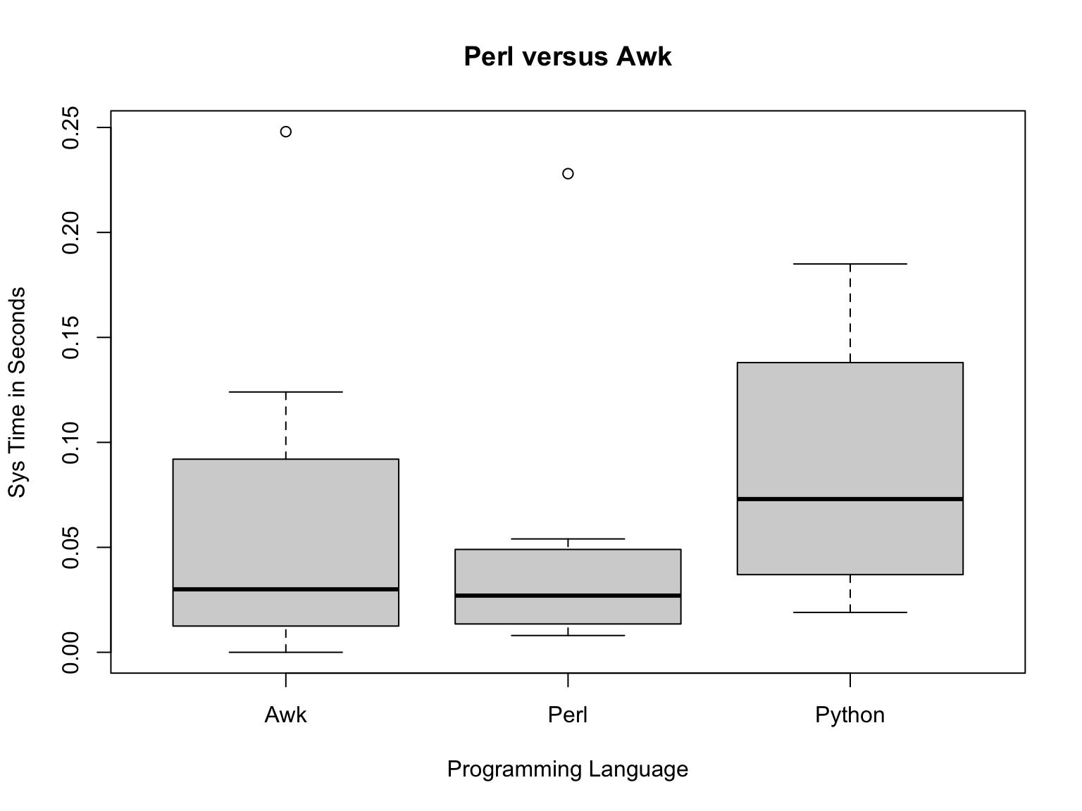
Now we can see the boxes a bit better and while we still have outliers, we’ve mostly removed the extremes.
From the boxplots, it looks like Awk is a bit slower than Perl, but let’s compare the means of each group:
## [1] 0.04375## [1] 0.06309091Notice this new way of subsetting from categorical data.
First, let’s look at the full size file results:
full=subset(pva2,pva2$Input.VCF.File.Size.=="Full")
plot(full$Programming.Language.,full$Sys.Run.Time.,main="Perl versus Awk for Full File",xlab="Programming Language",ylab="Sys Time in Seconds")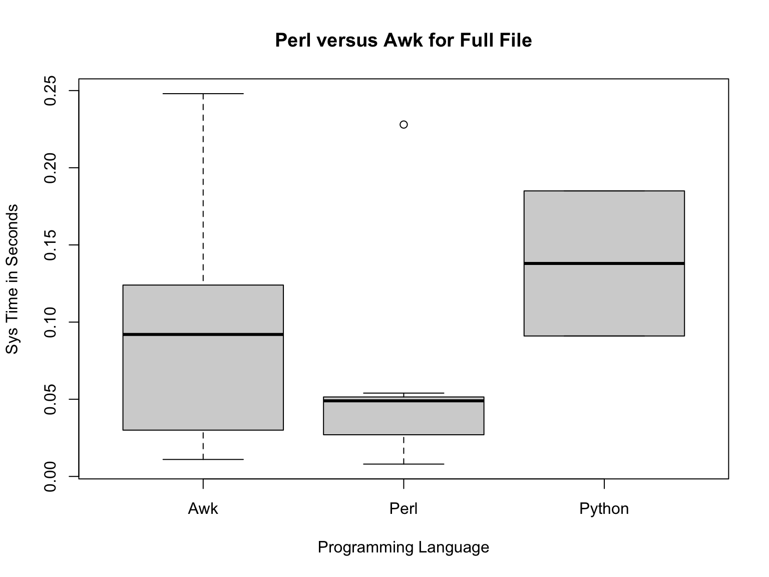
Here, Perl appears faster than Awk, with Python the slowest. But what
about for the smaller file when you used head to get only
the first 10,000 lines?
Now, let’s look at the small size fill results:
small=subset(pva2,pva2$Input.VCF.File.Size.=="Partial")
plot(small$Programming.Language.,small$Sys.Run.Time.,main="Perl versus Awk for Small File",xlab="Programming Language",ylab="Sys Time in Seconds")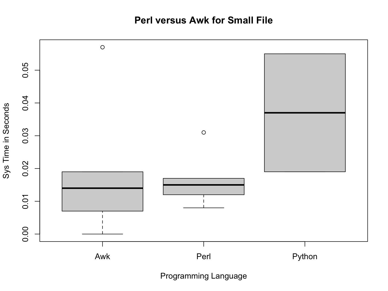
Now, Perl and Awk are pretty similar to each other and python is still the slowest.
## [1] 0.06314286## [1] 0.0995## [1] 0.0166## [1] 0.0194So, the means are different, but are they statistically different?
We can test this by using the function aov which fits
the data to an analysis of variance model. This calls the
lm function, which is for linear models.
model_full=aov(full$Sys.Run.Time.~full$Programming.Language.)
model_small=aov(small$Sys.Run.Time.~small$Programming.Language.)

#get AOV Table
summary(model_full)
## Df Sum Sq Mean Sq F value Pr(>F)
## full$Programming.Language. 2 0.01012 0.005058 0.815 0.466
## Residuals 12 0.07444 0.006204## Df Sum Sq Mean Sq F value Pr(>F)
## small$Programming.Language. 2 0.0006213 0.0003106 0.955 0.42
## Residuals 9 0.0029264 0.0003252Answer: NO! So, don’t do anything rash, like choose a particular language based on these data!
On your own: We also recorded OS in this dataset. On your own, compare the sys run time based on OS just like we did here using Programming Language. If you chose to read in the pre-existing object, remember to revisit the code we used to correctly code our categorical columns.
Basic Summary Statistics:
As we did before, let’s revisit some basic summaries of this dataset.
##       IDNO           BODYFAT         DENSITY           AGE            WEIGHT
##  Min.   :  1.00   Min.   : 0.00   Min.   :0.995   Min.   :22.00   Min.   :118.5
##  1st Qu.: 63.75   1st Qu.:12.80   1st Qu.:1.041   1st Qu.:35.75   1st Qu.:159.0
##  Median :126.50   Median :19.00   Median :1.055   Median :43.00   Median :176.5
##  Mean   :126.50   Mean   :18.94   Mean   :1.056   Mean   :44.88   Mean   :178.9
##  3rd Qu.:189.25   3rd Qu.:24.60   3rd Qu.:1.070   3rd Qu.:54.00   3rd Qu.:197.0
##  Max.   :252.00   Max.   :45.10   Max.   :1.109   Max.   :81.00   Max.   :363.1
##      HEIGHT        ADIPOSITY          NECK           CHEST           ABDOMEN
##  Min.   :29.50   Min.   :18.10   Min.   :31.10   Min.   : 79.30   Min.   : 69.40
##  1st Qu.:68.25   1st Qu.:23.10   1st Qu.:36.40   1st Qu.: 94.35   1st Qu.: 84.58
##  Median :70.00   Median :25.05   Median :38.00   Median : 99.65   Median : 90.95
##  Mean   :70.15   Mean   :25.44   Mean   :37.99   Mean   :100.82   Mean   : 92.56
##  3rd Qu.:72.25   3rd Qu.:27.32   3rd Qu.:39.42   3rd Qu.:105.38   3rd Qu.: 99.33
##  Max.   :77.75   Max.   :48.90   Max.   :51.20   Max.   :136.20   Max.   :148.10
##       HIP            THIGH            KNEE           ANKLE          BICEPS         FOREARM
##  Min.   : 85.0   Min.   :47.20   Min.   :33.00   Min.   :19.1   Min.   :24.80   Min.   :21.00
##  1st Qu.: 95.5   1st Qu.:56.00   1st Qu.:36.98   1st Qu.:22.0   1st Qu.:30.20   1st Qu.:27.30
##  Median : 99.3   Median :59.00   Median :38.50   Median :22.8   Median :32.05   Median :28.70
##  Mean   : 99.9   Mean   :59.41   Mean   :38.59   Mean   :23.1   Mean   :32.27   Mean   :28.66
##  3rd Qu.:103.5   3rd Qu.:62.35   3rd Qu.:39.92   3rd Qu.:24.0   3rd Qu.:34.33   3rd Qu.:30.00
##  Max.   :147.7   Max.   :87.30   Max.   :49.10   Max.   :33.9   Max.   :45.00   Max.   :34.90
##      WRIST          X
##  Min.   :15.80   Mode:logical
##  1st Qu.:17.60   NA's:252
##  Median :18.30
##  Mean   :18.23
##  3rd Qu.:18.80
## Max. :21.40## [1] 118.50 363.15## [1] 0.0 45.1Summary is a much more comprehensive view of this dataset.
In a previous video, you were asked to analyze this dataset on your own. Each of you did independent correlations of each variable and how it correlated with bodyfat. Because these were non-independent tests, we have to correct for multiple testing. However, a better way to compare how different parameters predict a response variable is to fit the data to a more complex model
#first, like aov, we will fit a generalized linear model:
fit=glm(BODYFAT~WEIGHT+DENSITY+ADIPOSITY+AGE+HEIGHT+NECK+CHEST+ABDOMEN+HIP+THIGH+KNEE+ANKLE+BICEPS+FOREARM+WRIST,data=fat)

#to see the fit, we will make a summary table
summary(fit)
##
## Call:
## glm(formula = BODYFAT ~ WEIGHT + DENSITY + ADIPOSITY + AGE +
## HEIGHT + NECK + CHEST + ABDOMEN + HIP + THIGH + KNEE + ANKLE +
## BICEPS + FOREARM + WRIST, data = fat)
##
## Deviance Residuals:
## Min 1Q Median 3Q Max
## -7.7632 -0.3308 -0.0954 0.2078 13.9487
##
## Coefficients:
## Estimate Std. Error t value Pr(>|t|)
## (Intercept) 4.190e+02 9.802e+00 42.750 <2e-16 ***
## WEIGHT 1.197e-02 1.467e-02 0.816 0.415
## DENSITY -3.816e+02 7.559e+00 -50.481 <2e-16 ***
## ADIPOSITY -5.493e-02 8.113e-02 -0.677 0.499
## AGE 1.078e-02 8.808e-03 1.224 0.222
## HEIGHT -1.782e-02 3.019e-02 -0.590 0.556
## NECK -2.062e-02 6.427e-02 -0.321 0.749
## CHEST 2.993e-02 2.856e-02 1.048 0.296
## ABDOMEN 2.260e-02 3.016e-02 0.749 0.454
## HIP 1.611e-02 4.023e-02 0.401 0.689
## THIGH 1.354e-03 3.980e-02 0.034 0.973
## KNEE -3.978e-02 6.705e-02 -0.593 0.554
## ANKLE -7.170e-02 6.073e-02 -1.181 0.239
## BICEPS -6.291e-02 4.688e-02 -1.342 0.181
## FOREARM 4.324e-02 5.447e-02 0.794 0.428
## WRIST 3.640e-02 1.480e-01 0.246 0.806
## ---
## Signif. codes: 0 '***' 0.001 '**' 0.01 '*' 0.05 '.' 0.1 ' ' 1
##
## (Dispersion parameter for gaussian family taken to be 1.359181)
##
## Null deviance: 15079.02 on 251 degrees of freedom
## Residual deviance: 320.77 on 236 degrees of freedom
## AIC: 809.95
##
## Number of Fisher Scoring iterations: 2Here, we have built a statistical model to show how body fat varies due to MULTIPLE parameters in the data.