Basic plotting to summarize data
Two ways of examining data are to make histogram plots of a vector within the dataset or to plot two of the vectors against each other:
hist(data$Population)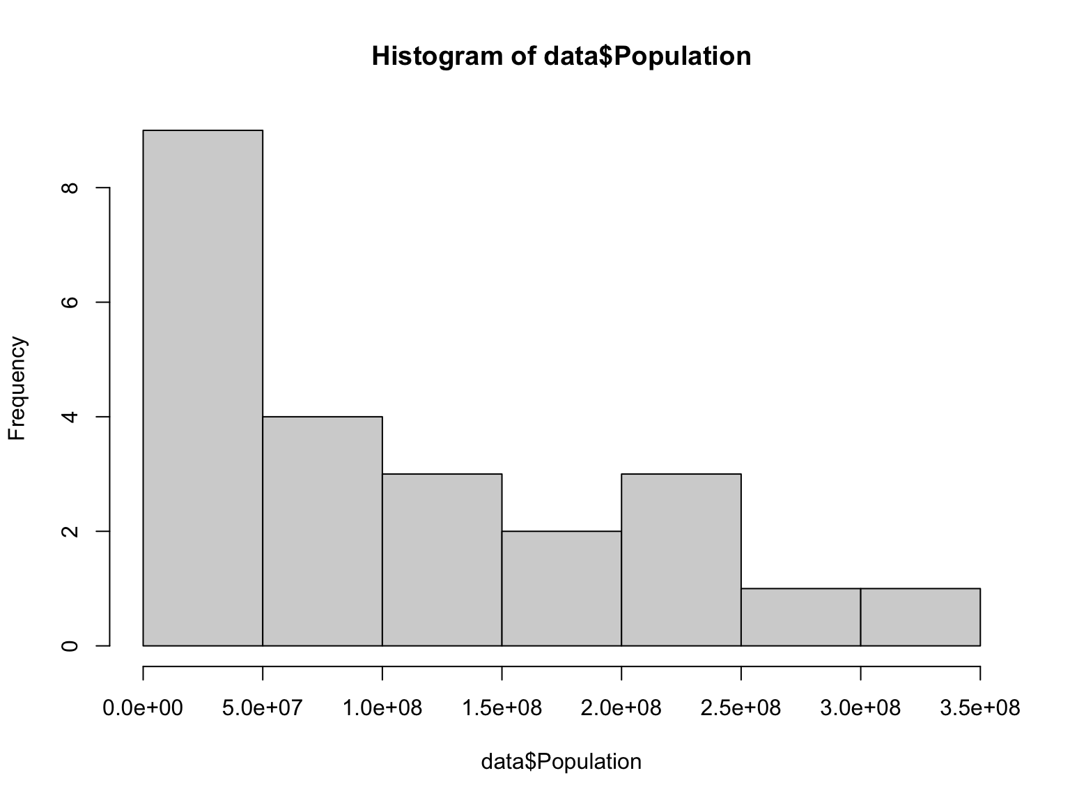
Laurie Stevison
If you are using this code with the video, note that some slides
have been added post-recording and are not shown. In this video we
will be working with two files in R: USpop.csv and
BodyFat.csv. Both files are available to download. Make an
R Notebook for this walk through tutorial to save all the code you will
be learning. We will cover:
mean and sdrangesummaryhist functionplot functionYou are working within an R project (check in the top right corner of RStudio - you should see the project name “R_Mini_Course”).
This means that the project directory will also be set as working directory. The exception is in a R Notebook, where the working directory is where the R Notebook is saved.
You should be saving your notebooks in the R Project and using
../.. to point at the main project directory.
Before starting, it may be helpful to have a chunk of code that does the following:
rm(list=ls())library(<package-name>)sessionInfo()list.files(getwd())## R version 4.2.1 (2022-06-23)
## Platform: x86_64-apple-darwin17.0 (64-bit)
## Running under: macOS Big Sur 11.7
##
## Matrix products: default
## LAPACK: /Library/Frameworks/R.framework/Versions/4.2/Resources/lib/libRlapack.dylib
##
## locale:
## [1] en_US.UTF-8/en_US.UTF-8/en_US.UTF-8/C/en_US.UTF-8/en_US.UTF-8
##
## attached base packages:
## [1] stats graphics grDevices utils datasets methods base
##
## other attached packages:
## [1] knitr_1.40 rmarkdown_2.17
##
## loaded via a namespace (and not attached):
## [1] digest_0.6.30 R6_2.5.1 jsonlite_1.8.3 magrittr_2.0.3 evaluate_0.18
## [6] highr_0.9 stringi_1.7.8 cachem_1.0.6 rlang_1.0.6 cli_3.4.1
## [11] rstudioapi_0.14 jquerylib_0.1.4 bslib_0.4.1 tools_4.2.1 stringr_1.4.1
## [16] xfun_0.34 yaml_2.3.6 fastmap_1.1.0 compiler_4.2.1 htmltools_0.5.3
## [21] sass_0.4.2## [1] "_site.yml" "4.02.Basic_Summary_Statistics_in_R_files"
## [3] "4.02.Basic_Summary_Statistics_in_R.html" "4.02.Basic_Summary_Statistics_in_R.Rmd"
## [5] "4.03.Data_Manipulation_in_R.Rmd" "4.04.Advanced_Statistical_Concepts_in_R.Rmd"
## [7] "4.05.R_on_CL.Rmd" "4.06.Programming_in_R.Rmd"
## [9] "5.03.Advanced_Graphing_in_R.Rmd" "about.Rmd"
## [11] "Activity1_intro.pdf" "activity1.html"
## [13] "activity1.Rmd" "activity1key.html"
## [15] "activity1key.Rmd" "activity2.html"
## [17] "activity2.Rmd" "activity3.html"
## [19] "activity3.Rmd" "Body_Fat.pdf"
## [21] "Congrats.html" "Congrats.Rmd"
## [23] "data" "docs"
## [25] "images" "index.html"
## [27] "index.Rmd" "LICENSE"
## [29] "module1.html" "module1.Rmd"
## [31] "module2.html" "module2.Rmd"
## [33] "module3.html" "module3.Rmd"
## [35] "module4.html" "module4.Rmd"
## [37] "module5.html" "module5.Rmd"
## [39] "module6.html" "module6.Rmd"
## [41] "module7.html" "module7.Rmd"
## [43] "modules" "R_Mini_Course.Rproj"
## [45] "raw_data" "README.md"
## [47] "README.Rmd" "site_libs"The first file contains 200 years of US census data.
You will need to add path information to the raw_data
directory once you have uncompressed the data tarball. Read the file
into an object called “data”:
You may also read in the previously made object into “data”:
To calculate the mean population size, you need to tell R to specifically look at the second column. Note the two different ways to specify the second column:
## [1] 103933744## [1] 103933744Next, we will cover some basic summary statistics of your new
dataset. These commands can be used to explore your data. Note
summary contains mean and range within it’s output.
## [1] 96177866## [1] 1790 2010## Min. 1st Qu. Median Mean 3rd Qu. Max.
## 3929214 20130664 75994575 103933744 165010268 308745538Two ways of examining data are to make histogram plots of a vector within the dataset or to plot two of the vectors against each other:

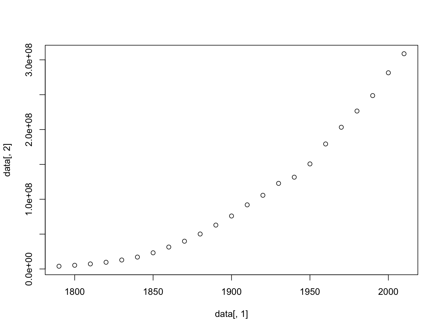
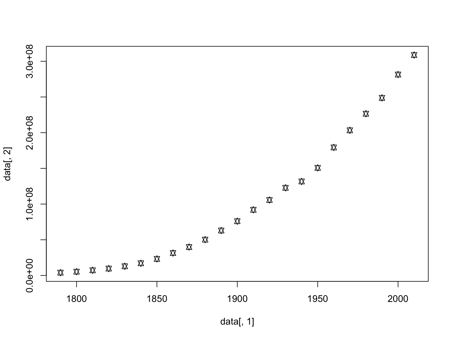
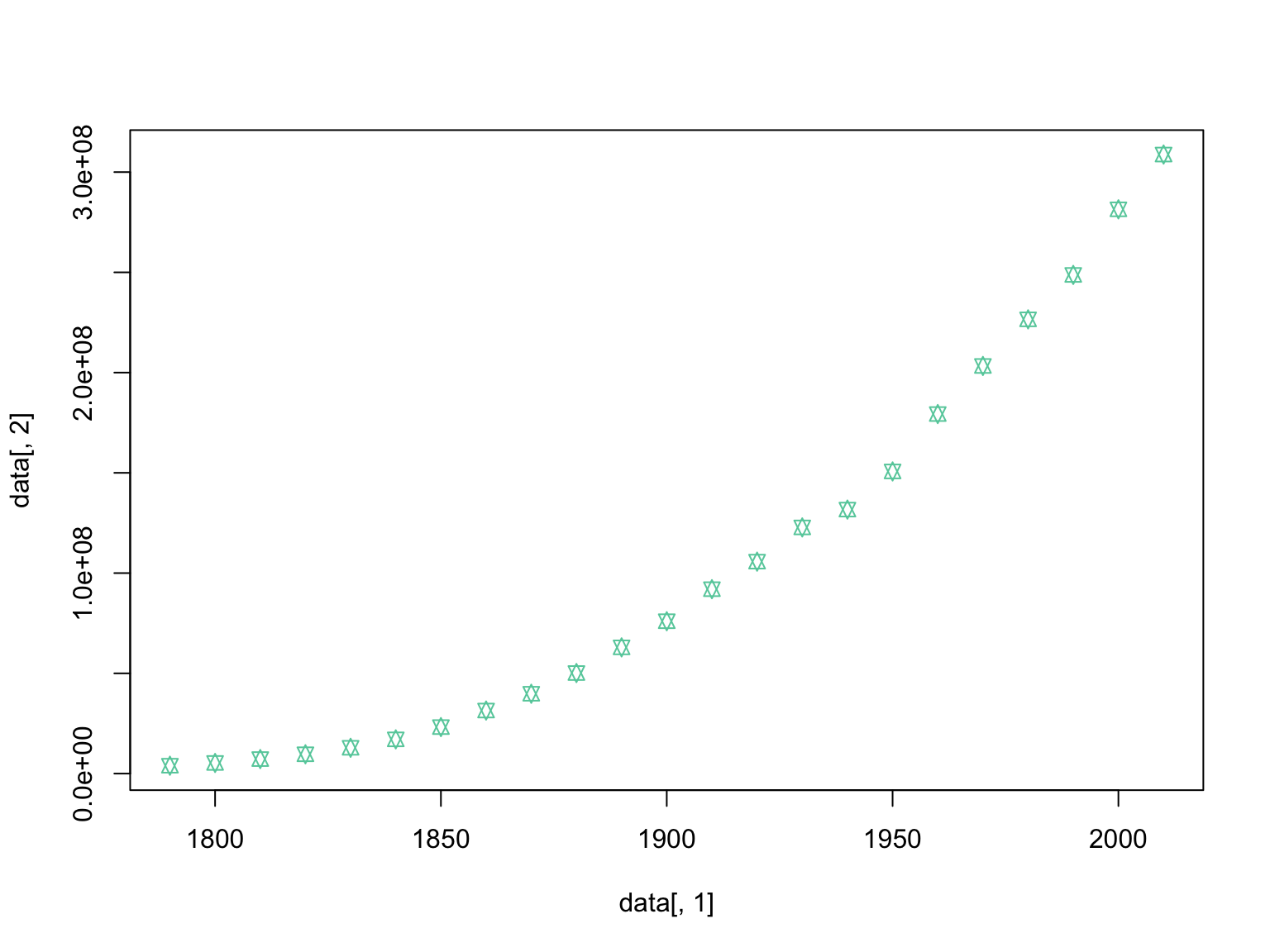
#change the size of the points relative to the plot
plot(data[,1], data[,2],pch=11, col="#66CDAA",cex=0.8)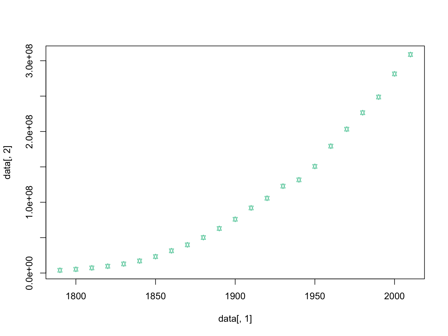
Next week we will learn how to make these plots look much nicer, but today we are focused on using them to visually inspect our data.
Some datasets can look very similar using simply summary statistics, but upon closer inspection using plots, they are indeed quite different. For this reason it is important to explore your datasets in both ways.
Anscombe’s quartet is a built in dataset within R. You can access it
by typing anscombe into your console:
| x1 | x2 | x3 | x4 | y1 | y2 | y3 | y4 |
|---|---|---|---|---|---|---|---|
| 10 | 10 | 10 | 8 | 8.04 | 9.14 | 7.46 | 6.58 |
| 8 | 8 | 8 | 8 | 6.95 | 8.14 | 6.77 | 5.76 |
| 13 | 13 | 13 | 8 | 7.58 | 8.74 | 12.74 | 7.71 |
| 9 | 9 | 9 | 8 | 8.81 | 8.77 | 7.11 | 8.84 |
| 11 | 11 | 11 | 8 | 8.33 | 9.26 | 7.81 | 8.47 |
| 14 | 14 | 14 | 8 | 9.96 | 8.10 | 8.84 | 7.04 |
| 6 | 6 | 6 | 8 | 7.24 | 6.13 | 6.08 | 5.25 |
| 4 | 4 | 4 | 19 | 4.26 | 3.10 | 5.39 | 12.50 |
| 12 | 12 | 12 | 8 | 10.84 | 9.13 | 8.15 | 5.56 |
| 7 | 7 | 7 | 8 | 4.82 | 7.26 | 6.42 | 7.91 |
| 5 | 5 | 5 | 8 | 5.68 | 4.74 | 5.73 | 6.89 |
Extract a corresponding set of x and y values from the dataset. Note the two possible ways to do this:
Now, as you did before, explore this dataset with mean summary statistics.
Compare the summary statistics of the set of x and y coordinates you had with others in your lab group (post a chat in MS teams in your private channel). Based on the summary statistics alone, how similar would you guess these datasets are?
##        x1             y1
##  Min.   : 4.0   Min.   : 4.260
##  1st Qu.: 6.5   1st Qu.: 6.315
##  Median : 9.0   Median : 7.580
##  Mean   : 9.0   Mean   : 7.501
##  3rd Qu.:11.5   3rd Qu.: 8.570
## Max. :14.0 Max. :10.840## [1] 3.316625## [1] 2.031568Make a histogram of the x and y sets. Then plot them against each other.
Again, compare the results of these tests with others in your lab group. Did the visual inspection of these datasets change your mind about how similar the four sets of data are in anscombe’s quartet?
Finally, let’s test for a statistical correlation between the x and y vectors.
##
##  Pearson's product-moment correlation
##
## data:  set1$x1 and set1$y1
## t = 4.2415, df = 9, p-value = 0.00217
## alternative hypothesis: true correlation is not equal to 0
## 95 percent confidence interval:
##  0.4243912 0.9506933
## sample estimates:
##       cor
## 0.8164205## cor
## 0.8164205Note the second time we run the command we only have it print the estimate.
Finally, let’s return to our US Census data. Looking back at the plot
of increase in population size per decade, we can compare the rate of
growth prior to the turn of the 19th century to afterward. We will use
the function subset to accomplish this task:
Now, we can make histograms of the population size in these two subsets of the original dataset:
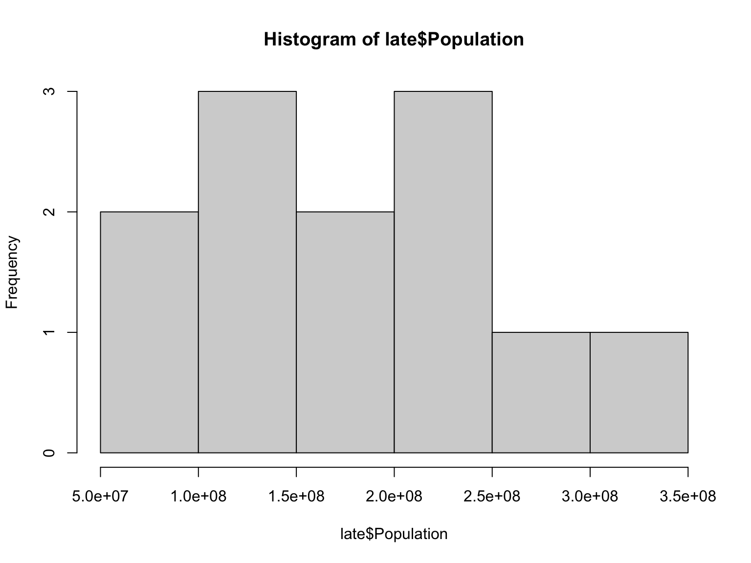
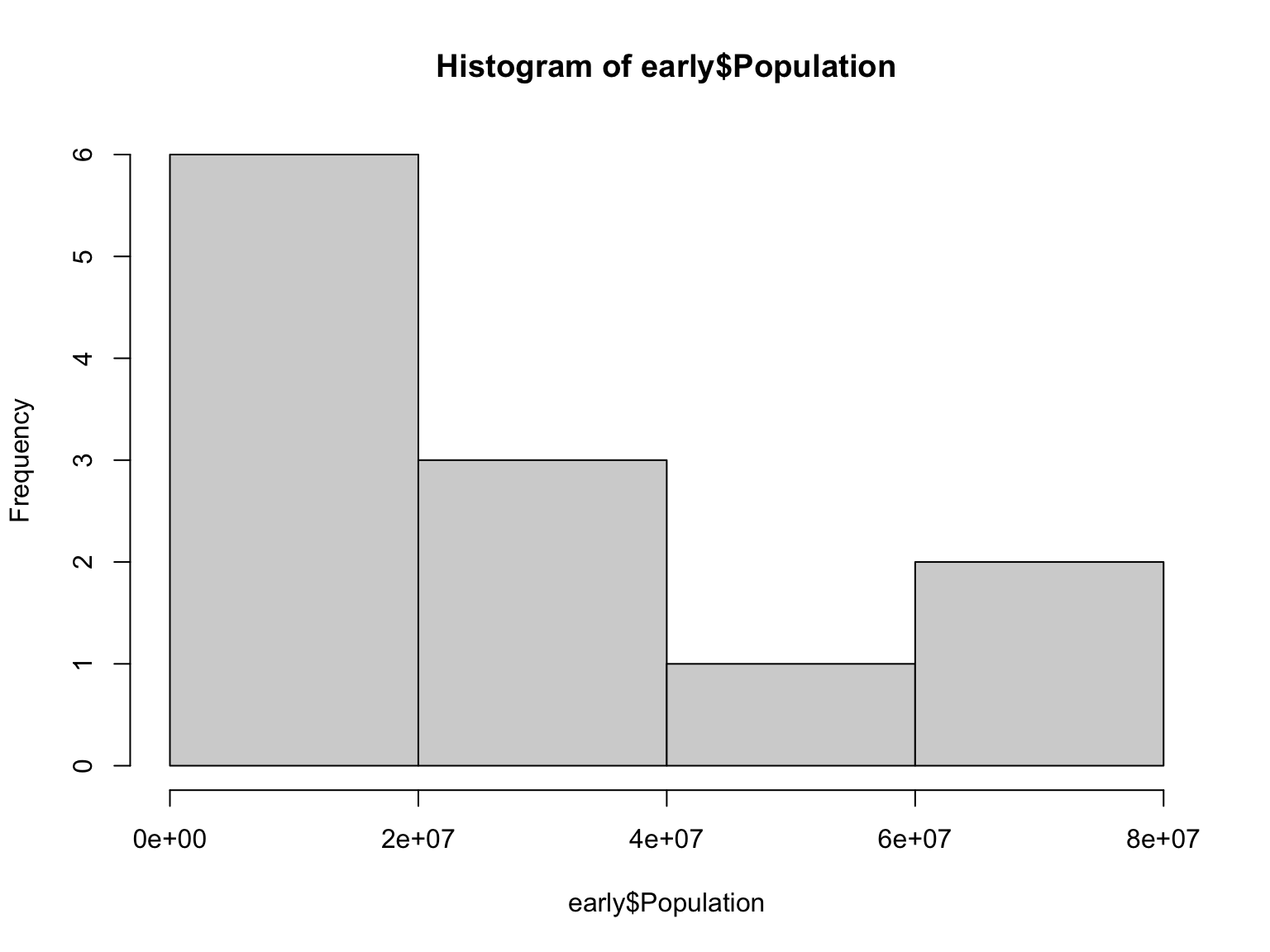
As we did before, let’s look at how the population size changed over time in these two distinct periods in US history:
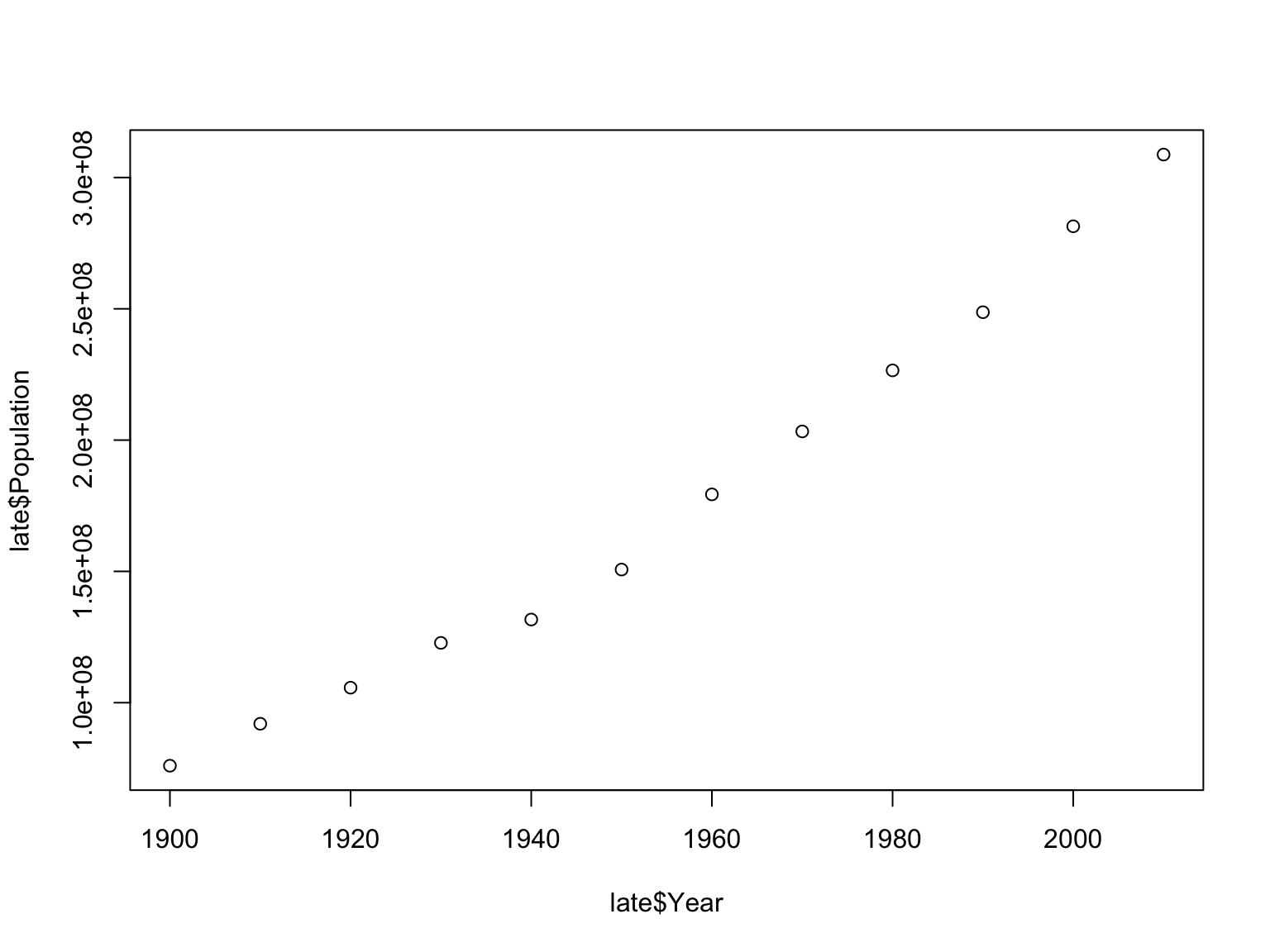
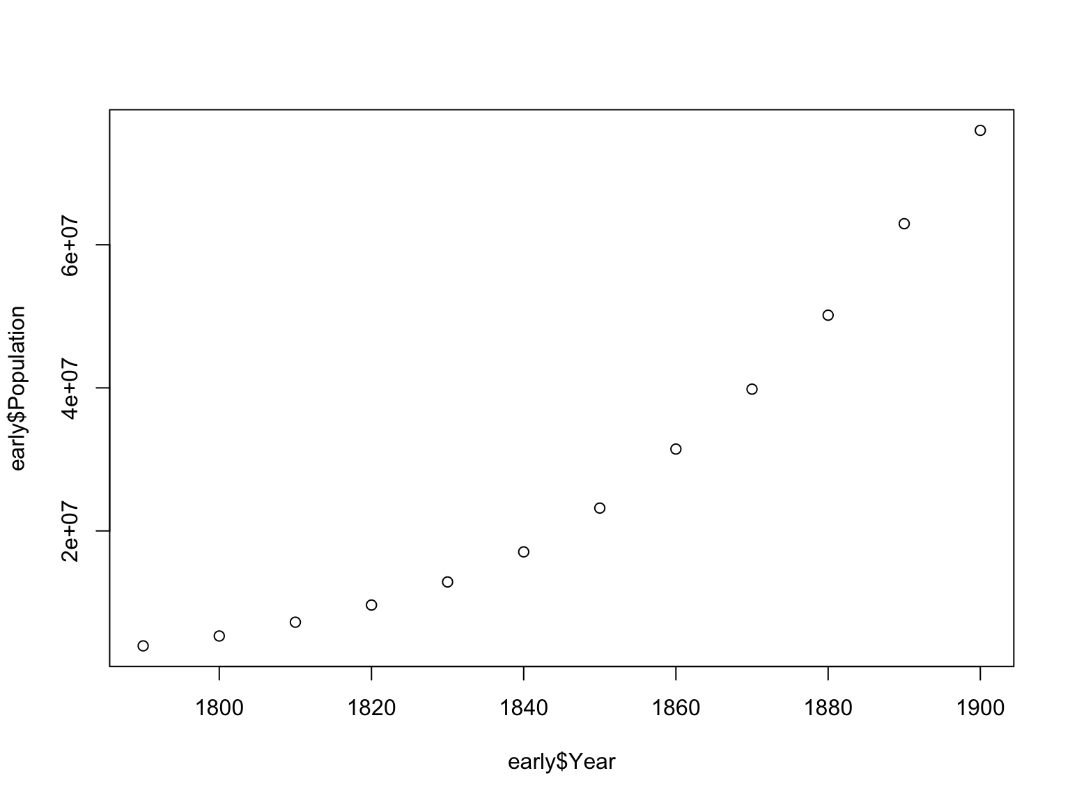

Let’s compare the growth of the US population between the early and the late periods. First, we can do a correlation test:
##
##  Pearson's product-moment correlation
##
## data:  early$Population and late$Population
## t = 17.543, df = 10, p-value = 7.7e-09
## alternative hypothesis: true correlation is not equal to 0
## 95 percent confidence interval:
##  0.9426362 0.9956808
## sample estimates:
##       cor
## 0.9841383##
## Spearman's rank correlation rho
##
## data: early$Population and late$Population
## S = 0, p-value < 2.2e-16
## alternative hypothesis: true rho is not equal to 0
## sample estimates:
## rho
## 1In the second example, we changed the default method from Pearson to Spearman. Why?
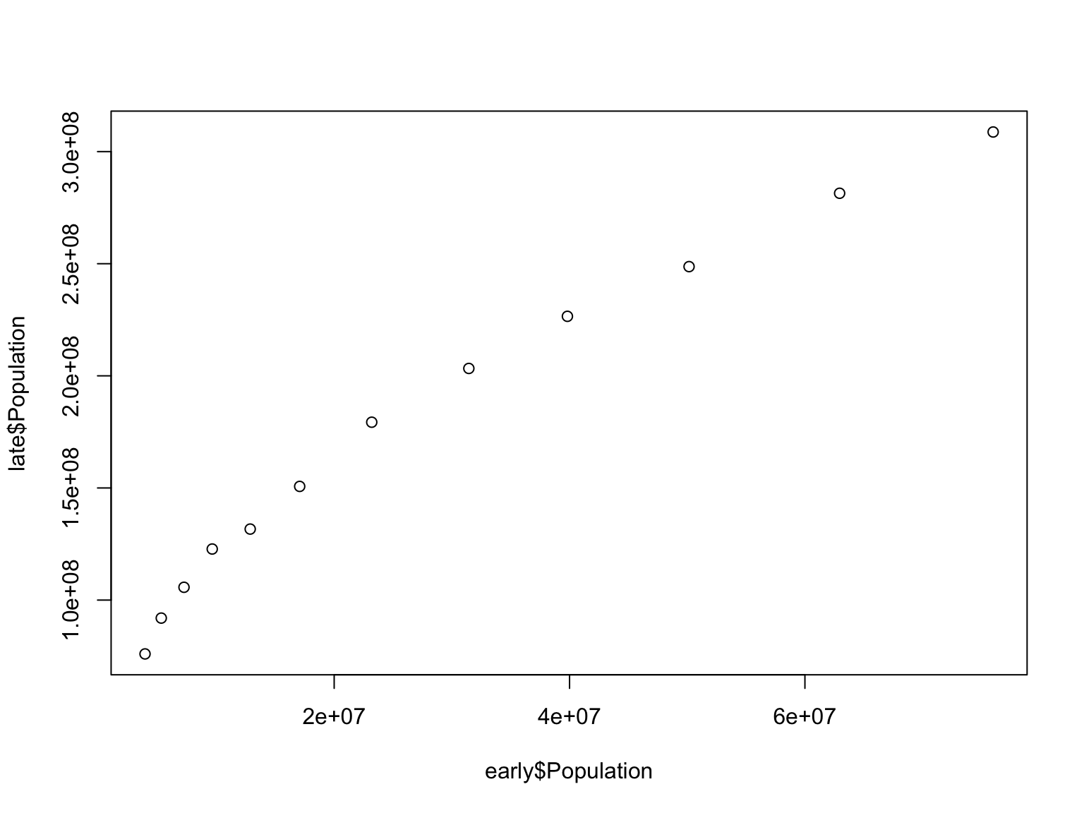
These are two different types of statistical correlation. The default is a Pearson correlation test, which expects a monotonic increase in the data, while a Spearman correlation is based on rank order.
To understand why the latter gives a better estimate, let’s look at these two growth periods together to better understand their relationship:
After finishing this video, work with the second dataset
BodyFat.csv. Follow the same process you did for the two
previous datasets:
fatCompare your results with others in your lab group.
Fill in the table below (see xlxs file now in your MS Teams channel
for your group) for each variable, the correlation estimate from
cor.test, and specify whether they correlate with body fat
based on the significance of the correlation.
| Variable | Correlation Estimate | Does it correlate with body fat? |
|---|---|---|
| DENSITY | Est: | Y | N |
| AGE | Est: | Y | N |
| WEIGHT | Est: | Y | N |
| HEIGHT | Est: | Y | N |
| ADIPOSITY | Est: | Y | N |
| NECK | Est: | Y | N |
| CHEST | Est: | Y | N |
| ABDOMEN | Est: | Y | N |
| HIP | Est: | Y | N |
| THIGH | Est: | Y | N |
| KNEE | Est: | Y | N |
| ANKLE | Est: | Y | N |
| BICEPS | Est: | Y | N |
| FOREARM | Est: | Y | N |
| WRIST | Est: | Y | N |